
Occlusion Aware Safety Augmentation for Partially Observed Reinforcement Learning
Abstract
Occlusion can hide scene information needed for safe action selection without changing the physical hazard. This manuscript develops COSA, a design for paired observation augmentation, visibility-sensitive representations, ensemble cost estimation, and constrained policy updates. Physical safety remains defined by a latent state-action cost; observation-dependent surrogates estimate that cost under partial observability. The proposed visual architecture is distinguished from a tested tabular realization on a 10×10 lava gridworld. The latter uses observation re-masking, additional Q-learning replay, a blended bootstrap penalty, and a runtime fallback. Across 20 training seeds allocated to five fixed maps, its reported severe-occlusion violation rate is 0.059 versus 0.341 for domain randomization and 0.152 for a belief-augmented baseline; its return is 0.766 versus 0.767 at k=0. Removing replay substantially reduces performance, while removing the fallback slightly improves it at k=2. These observations support the tabular combination on the tested maps. They do not validate learned visual encoders, calibrated uncertainty bounds, trust-region constraint guarantees, or transfer to new occluder classes.
Keywords:Safe reinforcement learningVisual reinforcement learningOcclusion robustnessCounterfactual data
augmentation, Constrained Markov decision process, Image inpainting.
1. Introduction
Consider a mobile manipulator that must retrieve a parcel from a shelf where neighbouring cartons partly cover the walking surface, or a delivery robot pulling away from a curb while a parked van screens the crosswalk behind it. In both situations, the visual observation available to the robot conceals exactly those scene elements that determine whether the next action is safe. Deep reinforcement learning agents that map camera images directly to actions have become strikingly capable in clean simulated scenes, yet their behaviour under cluttered, partially occluded viewing conditions remains difficult to predict. The difficulty is not marginal: in warehouses, hospitals, and domestic kitchens, occlusion is the normal condition of operation, not an exceptional disturbance. A policy that is safe when hazards are fully visible can become silently unsafe when they are hidden, because nothing in its training signal distinguishes a clear view from a misleading one. Safe reinforcement learning optimizes return subject to constraints on undesirable events [1–3]. Visual control and augmentation address learning from images and variation in rendering [4–9]. Defining physical cost as c(s,a) does not assume that the policy observes s. The difficulty here is inferring and controlling that cost when hazard-relevant information is obscured, including settings in which a simulator supplies privileged cost labels during training.
Occlusion removes selected visual information and may conceal a hazard. A hidden hazard remains physically present, and conservative behavior may be appropriate when its status cannot be inferred reliably. Generic corruption benchmarks [10–12] assess other forms of visual degradation; neither all corruptions nor all occlusions affect observations uniformly. Paired simulator views can isolate a specified observation edit, but their safety interpretation depends on preserving physical state and action.
COSA proposes minimal-edit observation pairs differing in hazard visibility while retaining the same physical state and action. The visual design combines cost supervision with visibility-sensitive representations and an uncertainty-inflated surrogate. Section 5 tests a tabular replay-and-penalty realization. It provides evidence for that computational combination rather than validation of the complete visual architecture.
The formal design separates latent physical cost from its observation-dependent estimate under partial observability (Section 3).
The proposed augmentation pipeline generates conceal-and-reveal observation pairs through simulator rendering or screened inpainting (Section 4.2).
Representation objectives distinguish hazard-irrelevant consistency from visibility discrimination; both paired views retain the same physical cost label. An ensemble spread term biases the proposed surrogate toward caution, without itself providing a calibrated bound (Sections 4.3 and 4.4).
The reported gridworld comparison evaluates tabular Q-learning variants over 20 seeds on five fixed maps, with four masking severity levels (Section 5).
The analysis states which architecture components are tested, which remain proposals, and which controls are required for causal attribution and generalization.
The remainder of the manuscript is organized as follows. Section 2 synthesizes related work across safe reinforcement learning, visual augmentation, and counterfactual image generation. Section 3 formalizes the problem and states the research questions and hypotheses. Section 4 develops the methodology, including the counterfactual generation pipeline, the representation objectives, and the constrained optimization scheme. Section 5 specifies the evaluation protocol, and Sections 6 and 7 discuss limitations, counterarguments, and future directions.
2. Related Work
2.1 Safe Reinforcement Learning and Constrained Policy Optimization
Constrained MDPs model return maximization subject to accumulated-cost constraints [1]. García and Fernández [2] survey safety criteria and exploration mechanisms. Constrained policy optimization establishes bounds and near-constraint satisfaction under its stated update assumptions [3], extending trust-region ideas [13]. Other algorithms and benchmarks offer alternative implementations [14–17]. These guarantees do not transfer automatically to an estimated-cost surrogate or a generic dual-ascent procedure.
Partial observability separates the true state from the information available to the policy. Belief-state planning provides a formal approach [18], while learned image encoders supply practical approximations. Simulator cost labels can train an estimator despite incomplete observations. The question is whether its error and uncertainty are controlled well enough for the intended safety constraint, rather than whether state-based physical cost is invalid.
2.2 Visual Reinforcement Learning and Augmentation-Based Generalization
Visual reinforcement learning includes control from pixels [4] and visuomotor policies [5]. Input augmentation can improve data efficiency and generalization [7], while DrQ regularizes value estimates through image augmentation [8]. Random Erasing creates rectangular occlusions for image-recognition training [19]; it does not by itself establish safe closed-loop behavior under hidden hazards. Domain and dynamics randomization [6], [20], rendered training [21], and procedural scene generation [9] supply other forms of variation. These works motivate the design without establishing that every generic augmentation fails to address hazards.
Corruption and distribution-shift benchmarks document visual fragility [10–12]. Their protocols differ from closed-loop safety evaluation, but this does not make them uniformly corrupted or categorically irrelevant. The present protocol focuses on masking hazard-relevant observations and measuring resulting policy outcomes.
2.3 Counterfactual Image Generation and Uncertainty Estimation
Simulator edits can change a rendering while preserving a specified latent state. Calling them counterfactual observations identifies that intervention; causal attribution requires the other relevant variables to remain fixed [22]. Image generation and inpainting methods provide possible editing tools [23–26], while diffusion models and view synthesis offer further design options [27–29]. Photorealism alone does not verify that the hazard state or its cost label has been preserved.
Ensemble disagreement is a practical uncertainty proxy [30], and dropout offers another approximation [31]. Neither spread nor a heatmap [32] proves calibration or safety. Encoder choices [33], [34] and auxiliary objectives [35] motivate the visual design. The assembled architecture requires separate implementation and validation; its novelty is framed as a proposed integration, without an exhaustive absence-of-prior-work claim.
2.4 Synthesis and Gap
Table 1 contrasts the selected works with the proposed design. These entries describe those works, not every member of each method family. The visual COSA row states design capabilities; the experiments test a distinct tabular combination. Paired data, uncertainty-aware cost estimation, and constrained updates must each be evaluated before the full integration can be claimed effective.
Table 1. Design capabilities of selected works and the proposed visual architecture. The COSA row describes proposed components, not components executed by the tabular study.
This table is shown in the PDF version of the article.
3. Problem Formulation and Research Questions
The physical task is a constrained process observed through a lossy rendering channel. The formal design and its tabular realization answer different levels of the research questions; Section 5 specifies the limited empirical coverage.
3.1 Research Questions and Hypotheses
The questions concern cost estimation under hidden hazards, the value of paired training views, and uncertainty-based conservatism. The hypotheses below are proposed tests. The tabular campaign does not execute learned encoder, calibrated-ensemble, or held-out-occluder evaluations.
RQ1 asks how to estimate latent physical safety cost from observations that hide hazard-relevant state, and how to calibrate uncertainty about that estimate.
RQ2 asks whether paired observation edits improve representations and safety compared with unpaired edits at matched data and optimizer-update budgets.
RQ3 asks whether uncertainty inflation adapts conservatism to masking severity and transfers to occluder classes absent from training.
H1 predicts lower violation rates from the proposed surrogate under occluded evaluation, relative to a comparator with matched learning and observation conditions.
H2 predicts improved held-out-occluder generalization from paired versus unpaired augmentation. That test is not executed here.
H3 predicts that calibrated uncertainty inflation changes behavior with severity. The tested tabular penalty is not an ensemble-uncertainty implementation of this hypothesis.
3.2 System Model and Notation
Let M=(S,A,P,r,c,γ,μ₀) describe the physical constrained process. The policy receives oₜ=R(sₜ,ωₜ) rather than sₜ, so the observation model makes the decision problem partially observable. The occluder configuration ωₜ affects rendering only. Physical hazard cost c(s,a) is unchanged by observation edits; κ(o,a) is an estimate used by the agent. History-dependent policies or beliefs may be needed because an individual observation need not be Markov. Table 2 collects the notation.
Table 2. Notation used throughout the manuscript.
This table is shown in the PDF version of the article.
f_k(o, a) k-th member of the cost-estimator ensemble mu_hat_K, sigma_hat_K Ensemble mean and standard deviation of cost estimates kappa_bar(o, a) Uncertainty-inflated surrogate cost, Eq. (2) beta Uncertainty-inflation coefficient d Expected-cost budget in Eq. (1) lambda Dual variable of the constrained update D_cf Buffer of factual-counterfactual observation pairs L_pair, L_disc Consistency and visibility-discrimination losses in the proposed visual design, Eq. (3)
3.3 Formal Problem Statement
The physical goal is to maximize expected discounted return while bounding expected discounted latent cost. The proposed optimizer instead bounds a surrogate built from ensemble mean and spread. Eq. (1) states this surrogate constraint. It implies a physical-cost bound only if the surrogate conservatively covers the relevant latent cost or a suitable error bound is incorporated. Agreement among ensemble members does not ensure that condition. A positive β term biases estimated cost upward relative to its mean, but common-mode errors can remain.
t (1)
Jκ ‾ (θ) = π [∑ γ κ ‾(ot, at)] ≤ d.
κ ‾(o, a) = μ ̂K(o, a) + βσ ̂K(o, a).
2 (3)
ℒenc = ℒpair + αℒdisc, ℒpair =∥ zirr(o) − zirr(ocf) ∥ .
In Eq. (3), zirr denotes a hazard-irrelevant representation head. Its consistency loss preserves content that should be unaffected by the observation edit. Ldisc discriminates visibility status using renderer-derived mask labels, rather than imposing different physical cost targets. A separate cost-regression objective assigns both paired views the same c(s,a). These objectives form a proposed design; their calibration and interaction are not tested by the tabular experiments.
4. Proposed Methodology
4.1 Overview and Assumptions
The visual design has a paired-observation generator, encoder, ensemble cost estimator, and constrained policy optimizer. Training would interleave rollouts and edited observations. Simulator masks and physical cost labels provide supervision, while inference uses available observations. Algorithm 1 specifies the proposed loop; its neural and constrained-update components are not implemented in Section 5.
Training requires a simulator exposing rendering, depth, and object masks for controlled observation edits. The physical latent cost must be computable for simulator supervision even when the policy cannot observe the hazard. Occlusion edits are assumed to affect observations only; physical state, transition dynamics, and cost labels remain fixed. Simulator re-rendering or screened inpainting must preserve the intended latent state. Visual plausibility alone is insufficient. The design assumes a single camera. Additional sensing or active viewpoints are possible extensions.
4.2 Counterfactual Scene Generation
A reveal edit removes a visual occluder and a conceal edit inserts one, while preserving physical state, action, and non-designated scene factors. Simulator rendering is preferred when it permits those controls. Inpainting [25], [26] and diffusion-based generation [27] are possible alternatives, but they can introduce artifacts or change inferred scene content. A taxonomy of occluder classes is a proposed extension; the tabular study uses only rectangular masking.
Pairs are annotated with a mask and a visibility measure, such as the fraction of hazard area covered. A pixel audit checks non-designated regions, and a state audit checks that physical hazards and costs are unchanged. Both observations receive the same c(s,a) target. These controls define the observation intervention; they do not by themselves isolate its learning effect from additional data or updates.
Algorithm 1. COSA training loop.
Input: simulator G with segmentation access; latent cost c(s, a); ensemble size K; inflation coefficient beta; pair-generation probability p_cf; expected-cost budget d 1: initialize policy pi_theta, encoder g_psi, cost ensemble f_1..f_K, dual variable lambda 2: repeat 3: collect rollout batch B with pi_theta in G 4: for each transition (o_t, a_t, s_t) in B do 5: with probability p_cf sample occluder config omega' and occlusion intensity rho 6: o_cf <- composite(G, s_t, omega') or inpaint(o_t, mask) 7: run mask audit and perceptual screening; discard on failure 8: store (o_t, o_cf, mask, visibility, c(s_t, a_t)) in D_cf 9: end for 10: update the encoder with irrelevant-content consistency and visibility discrimination 11: regress each paired cost prediction to the same physical c(s_t, a_t) 12: kappa_bar <- mu_hat_K + beta * sigma_hat_K // Eq. (2) 13: update pi_theta by constrained trust-region step on (J_r, J_c(kappa_bar)) with dual ascent on lambda // Eq. (1) 14: until training budget exhausted Output: policy pi_theta, encoder g_psi, cost ensemble f_1..f_K, fitted dual variable lambda
4.3 Occlusion-Aware Representation Objectives
The encoder uses separate heads for hazard-irrelevant content and visibility-relevant features. A consistency term is applied to the irrelevant head, while renderer-derived visibility labels guide Ldisc on the relevant head. Concealing a hazard does not change the underlying hazard state or its c(s,a) value. Thus cost estimates should target the same physical label for a conceal-and-reveal pair, although uncertainty may differ. Any measured distinction in prediction must be interpreted through estimator accuracy and calibration, not forced difference in true costs.
4.4 Uncertainty-Inflated Cost Estimation and Constrained Optimization
The K cost estimators are supervised by simulator costs. Their standard deviation is used as an uncertainty proxy in Eq. (2), rather than a certified upper bound. A constrained trust-region or Lagrangian implementation may optimize Jr−λ(Jc−d) [3], [15], but dual ascent alone does not ensure convergence or physical constraint satisfaction. Validation must assess cost-prediction error, spread calibration, feasibility, and realized physical costs under shifts. These checks are requirements for the proposed visual implementation; the tabular study does not perform them.
4.5 Complexity, Scalability, and Failure Conditions
Generation costs grow with the number of edits, and ensemble scoring grows with K. Pair storage adds memory and replay adds optimizer work. Inpainting, encoder training, calibration, and policy updates contribute further costs. The tabular campaign quantifies neither the neural overhead nor a compute-matched benefit of the full architecture.
The following are anticipated failure modes and proposed mitigations, rather than controls all executed by the present study:
I. Inpainting artifacts may become shortcuts; simulator rendering, region audits, and artifact controls can reduce this risk.
II. Synthetic occluders may differ from real clutter. Held-out-class and physical-scene tests remain necessary. III. Ensemble agreement may conceal shared errors. Calibration and realized-cost audits are required.
IV. Conservatism may reduce return or impede deadlines. A return–cost frontier should be measured across β and budget choices.
V. Counterfactual replay can add supervision for occluded views, but it must retain the same physical state-action cost label.
5. Experimental Results and Analysis
5.1 Setup
All experiments run on a purpose-built 10 x 10 gridworld navigation task implemented in NumPy. Each of the five fixed maps contains twelve lava cells, a goal in the top-right region, and episode starts drawn uniformly from the bottom-left region; stepping costs -0.01, reaching the goal yields +1.0 and terminates the episode with success, and entering lava yields -1.0 and terminates it with a safety violation, with episodes capped at 200 steps. The agent observes an egocentric 5 x 5 view plus four goal-direction bits, and occlusion is applied as k random 2 x 2 patches of the view masked per step, with a 5% per-step blackout probability retained at every occlusion level. The five maps were generated once with a fixed master seed and every training seed is assigned to one of them, so map layout acts as a controlled blocking factor.
Four tabular Q-learning agents [36] share the same state abstraction: agent position, coarse goal sector, four orthogonal-neighbour flags in {unknown, safe, hazard, wall}, and a caution bucket that coarsens the fraction of the local window that is currently unobserved. The naive baseline trains entirely on clean views; the domain-randomization baseline draws k uniformly from {0, ..., 4} each episode [6]; the belief-augmented baseline replaces last-seen flags with a persistent per-episode memory map that encodes unseen cells as hazards; and COSA trains on clean views while replaying every experienced transition under counterfactually re-masked observations (k' drawn from {1, 2, 4}) with a conservative bootstrap that blends the clean and occluded next-state values with weight lambda = 0.5, together with a risk-threshold fallback (tau = 0.15) that switches to a widest-margin detour action whenever the value gap between the observed and the worst-case state exceeds the threshold. All agents use alpha = 0.2, gamma = 0.95, and an epsilon schedule decaying linearly from 1.0 to 0.05.
The campaign reports 20 training seeds, assigned as four repeats on each of five fixed maps, and 3,000 training episodes per seed. Each policy is evaluated for 200 episodes at k∈{0,1,2,4}, using paired streams. Pilot training increased the episode budget from 600; no preregistration record is established. The stated runtime is 367.5 s, with Python 3.12, NumPy 2.1.3, SciPy 1.14.1, statsmodels 0.14.5 [37], and matplotlib 3.9.2. Exact reproduction requires the maps, streams, code, and outputs; variance and experimental reporting warrant careful control in reinforcement learning [38]. Matching episodes does not match additional replay updates or total compute. Absolute position in the state abstraction also permits map memorization; no map is held out.
5.2 Main Comparison (RQ1)
Tables 3 and 4 report returns and outcome rates over the 20 seeds. At k=1 the source reports naive return −1.133 and violation rate 0.994, whereas domain randomization and the belief baseline perform better. At k=4, domain randomization has return 0.056 and violation rate 0.341, and the belief baseline has return 0.463 and violations 0.152. These observations concern these implementations on five fixed maps. Unknown-state behavior is a plausible explanation for naive failure, but identifying it requires Q-table and action-trace inspection.
Table 3. Mean episode return (+/- std over 20 seeds) by policy and occlusion level k.
This table is shown in the PDF version of the article.
Each cell aggregates 200 test episodes per seed on shared evaluation streams.
levels k = 0, 2, and 4.
Policy Success k = 0 Success k = 2 Success k = 4 Naive Q (clean-trained) 0.945 +/- 0.022 0.002 +/- 0.003 0.010 +/- 0.012 Domain randomization 0.941 +/- 0.022 0.682 +/- 0.102 0.659 +/- 0.092 Belief-augmented Q 0.936 +/- 0.021 0.913 +/- 0.025 0.848 +/- 0.036 COSA (proposed) 0.944 +/- 0.019 0.932 +/- 0.024 0.941 +/- 0.023
5.3 Ablation of COSA Components (RQ2)
and seed controls.
COSA Variant (K = 2) Return Full COSA 0.749 +/- 0.047 Minus counterfactual augmentation -1.134 +/- 0.045 Minus conservative penalty 0.717 +/- 0.039 Minus risk fallback 0.759 +/- 0.051 k = 2 k = 4 -1.139 +/- 0.041 -1.143 +/- 0.045 0.069 +/- 0.231 0.056 +/- 0.205 0.664 +/- 0.053 0.463 +/- 0.077 0.749 +/- 0.047 0.766 +/- 0.044
Violation k = 0 Violation k = 2 Violation k = 4 0.055 +/- 0.022 0.998 +/- 0.003 0.990 +/- 0.012 0.059 +/- 0.022 0.317 +/- 0.103 0.341 +/- 0.091 0.064 +/- 0.021 0.086 +/- 0.025 0.152 +/- 0.036 0.056 +/- 0.019 0.068 +/- 0.024 0.059 +/- 0.023
Success Rate Violation Rate 0.932 +/- 0.024 0.068 +/- 0.024 0.020 +/- 0.011 0.980 +/- 0.011 0.925 +/- 0.020 0.075 +/- 0.020 0.937 +/- 0.026 0.063 +/- 0.026
Table 4. Success rate and safety-violation rate (+/- std over 20 seeds) by policy at occlusion
This table is shown in the PDF version of the article.
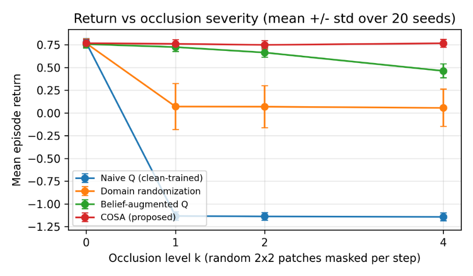
COSA reports k=4 return 0.766 and violation rate 0.059. The source traces describe a cautious Q-function, but the comparisons do not isolate that explanation from masked-state coverage or additional replay updates. The naive method has slightly higher k=0 return, so COSA does not dominate every cell. The runtime fallback and blended target are specific implementation choices, not a calibrated ensemble cost model.
Table 5 compares tabular variants at k=2. Removing re-masked replay leaves return −1.134 and violations 0.980; this changes both masked-state coverage and replay updates, so it does not isolate causal pairing. Removing the blended penalty changes return from 0.749 to 0.717 and violations from 0.068 to 0.075. The reported differences are consistent with a benefit of that variant at this level, subject to the common update Removing the fallback gives return 0.759 and violations 0.063, slightly better than the full method at k=2. Its protective effect is therefore not demonstrated at this severity. Unseen severities could test its intended role, but that remains an extension. The replay-removal contrast supports the complete replay treatment relative to its absence; a matched-update unpaired replay comparator is required to isolate pairing.
Table 5. Component ablation of COSA at occlusion level k = 2 (mean +/- std over 20 seeds): Return, success rate, and violation rate.
This table is shown in the PDF version of the article.
5.4 Robustness across Occlusion Levels (RQ3)
Fig. 2 and Table 4 show COSA violations near 0.06 across the tested levels, with belief-baseline violations increasing from 0.064 at k=0 to 0.152 at k=4, and domain randomization from 0.059 to 0.341. COSA success changes from 0.944 to 0.941. Here k=0 means no patch masking but retains a 5% blackout probability, so it is not a fully unobscured condition.
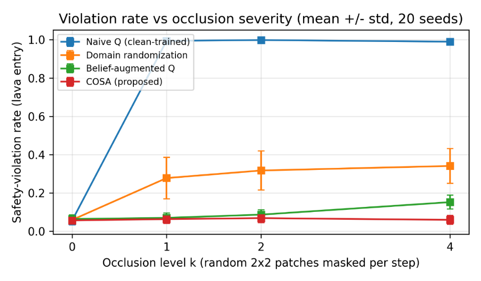
Every level retains 5% blackout; COSA is approximately flat over the tested levels.
Only one rectangular-mask mechanism is tested. Held-out occluder classes under H2 and calibrated ensemble inflation under H3 remain untested. A nearly flat violation profile is an observation of the tabular realization, not evidence that the proposed ensemble adapts uncertainty correctly.
5.5 Statistical Analysis
Table 6 retains paired-seed Wilcoxon [39], Holm [40], and Friedman [41] summaries. For k=4, the reported COSA-versus-randomization return contrast has W=0 and p=1.9e−6; the two-sided all-same-sign exact value is 2/2²⁰≈1.907e−6 under 20 independent nonzero pairs. The reported Friedman χ²(3)=60 is the maximum n(k−1) for n=20 and four methods without rank inconsistencies. Raw ranks, ties, and Holm family must be checked. The 20 seeds reuse five maps, so tests are conditional on this map set and do not establish generalization to independent environments.
Table 6. Statistical tests on the k = 4 evaluation cells (paired over 20 seeds; alpha = 0.05; Holm correction over the secondary family).
This table is shown in the PDF version of the article.
5.6 Discussion: Findings, Losses, and Scope
The tabular replay-and-penalty combination has lower reported violations under severe masking than the compared implementations. The penalty-removal contrast has a smaller difference, while the fallback-removal contrast slightly favors removal at k=2. COSA return at k=4 is close to its own k=0 value. These comparisons support the tested combination, but unmatched replay updates prevent attributing the main gain solely to paired observation structure.
At k=0, where patch masks are absent but 5% blackout remains, the naive policy has return 0.773 versus 0.767 for COSA and success 0.945 versus 0.944. The belief baseline remains competitive at mild masking. The fallback-removal variant is slightly better at k=2, and any protective effect beyond the trained range remains untested.
The tabular realization replaces image editing with view re-masking, neural cost uncertainty with a blended bootstrap, and constrained trust-region updates with a penalty in the TD target. It does not test the visual architecture. A 100-cell environment, one hazard class, one masking mechanism, and five reused maps provide limited evidence. Photorealistic and continuous-control transfer [42], new maps, encoder behavior, and physical constraint calibration remain open.
The reported observations are proof-of-concept results from the stated gridworld configuration. Code, maps, seeds, and raw outputs are required to establish their traceability and reproducibility.
6. Discussion: Limitations and Counterarguments
6.1 Limitations
The visual design depends on simulator supervision and state-preserving observation edits. Expected additive cost does not capture every irreversible safety concern. Ensemble disagreement may be miscalibrated under occlusion, and that calibration is not tested by this tabular study. Real-time overhead, deadlines, multiple sensors, and active viewpoint control also remain outside the evaluation.
6.2 Alternative Viewpoints and Responses
Domain randomization, memory-based beliefs, and paired replay are reasonable alternatives with different implementations. The reported randomization result does not settle which succeeds at matched update counts, observation coverage, or tuning budgets. A per-episode memory map is the strongest tested baseline under severe masking. Physical-scene validity of simulator edits and held-out occluder generalization require separate experiments.
7. Conclusion and Future Directions
COSA separates unchanged physical hazard cost from its observation-dependent estimate and proposes a visual architecture for paired edits and conservative cost modeling. The tabular realization reports approximately 6% violations across the tested masking levels, compared with larger severe-masking rates for the selected baselines. Replay removal strongly changes performance, but also changes data coverage and updates. The fallback adds no measured benefit at k=2. The experiment supports a scoped tabular combination; learned visual safety, calibrated ensemble inflation, and causal attribution to pairing remain untested.
Next tests should match replay updates and masked-state coverage, hold out maps and occluder classes, and establish traceability of the reported runs. A visual implementation must separately evaluate encoder heads, same-cost paired supervision, calibration, realized physical constraints, and runtime before transfer to real clutter.
Funding
This research received no specific grant from any funding agency in the public, commercial, or not-for-profit sectors.
Data Availability
The study uses a generated gridworld rather than an external dataset. The map realizations, seeds, evaluation streams, and raw outputs are necessary for reproducibility; a repository identifier is not specified.
Code Availability
A public repository and archived version for the reported implementation are not specified.
Conflicts of Interest
The authors declare no conflicts of interest.
Author Contributions
A. D.: study design, methodology, and original drafting. K. A. M.: Implementation, experiments, analysis, and review—editing. All authors approved the final version.
Generative AI Disclosure
AI-assisted drafting tools were used in preparing the manuscript text under the direction and scientific responsibility of the authors; all methodological choices, executed experiments, claims, and final content were determined and verified by the authors.
References
- [1] Altman, E. (2021). Constrained Markov decision processes. Routledge. https://doi.org/10.1201/9781315140223
- [2] Garcıa, J., & Fernández, F. (2015). A comprehensive survey on safe reinforcement learning. Journal of machine learning research, 16(1), 1437–1480. https://www.jmlr.org/papers/volume16/garcia15a/garcia15a.pdf
- [3] Achiam, J., Held, D., Tamar, A., & Abbeel, P. (2017). Constrained policy optimization. International conference on machine learning (pp. 22–31). PMLR. https://proceedings.mlr.press/v70/achiam17a
- [4] Mnih, V., Kavukcuoglu, K., Silver, D., Rusu, A. A., Veness, J., & Bellemare, M. G. (2015). Human-level control through deep reinforcement learning. Nature, 518(7540), 529–533. https://doi.org/10.1038/nature14236
- [5] Levine, S., Finn, C., Darrell, T., & Abbeel, P. (2016). End-to-end training of deep visuomotor policies. Journal of machine learning research, 17(39), 1–40. https://www.jmlr.org/papers/v17/15-522.html
- [6] Tobin, J., Fong, R., Ray, A., Schneider, J., Zaremba, W., & Abbeel, P. (2017). Domain randomization for transferring deep neural networks from simulation to the real world. 2017 IEEE/rsj international conference on intelligent robots and systems (IROS) (pp. 23–30). IEEE. https://doi.org/10.1109/IROS.2017.8202133
- [7] Laskin, M., Lee, K., Stooke, A., Pinto, L., Abbeel, P., & Srinivas, A. (2020). Reinforcement learning with augmented data. Advances in neural information processing systems, 33, 19884–19895. https://doi.org/10.48550/arXiv.2004.14990
- [8] Kostrikov, I., Yarats, D., & Fergus, R. (2020). Image augmentation is all you need: Regularizing deep reinforcement learning from pixels. https://doi.org/10.48550/arXiv.2004.13649
- [9] Cobbe, K., Hesse, C., Hilton, J., & Schulman, J. (2020). Leveraging procedural generation to benchmark reinforcement learning. International conference on machine learning (pp. 2048-2056). PMLR. https://proceedings.mlr.press/v119/cobbe20a.html
- [10] Hendrycks, D., & Dietterich, T. (2019). Benchmarking neural network robustness to common corruptions and perturbations. https://doi.org/10.48550/arXiv.1903.12261
- [11] Michaelis, C., Mitzkus, B., Geirhos, R., Rusak, E., Bringmann, O., Ecker, A. S., … & Brendel, W. (2019). Benchmarking robustness in object detection: Autonomous driving when winter is coming. https://doi.org/10.48550/arXiv.1907.07484
- [12] Hendrycks, D., Zhao, K., Basart, S., Steinhardt, J., & Song, D. (2021). Natural adversarial examples. Proceedings of the IEEE/CVF conference on computer vision and pattern recognition (pp. 15262–15271). https://doi.org/10.48550/arXiv.1907.07174
- [13] Schulman, J., Levine, S., Abbeel, P., Jordan, M., & Moritz, P. (2015). Trust region policy optimization. International conference on machine learning (pp. 1889–1897). PMLR. https://proceedings.mlr.press/v37/schulman15.html
- [14] Amodei, D., Olah, C., Steinhardt, J., Christiano, P., Schulman, J., & Mané, D. (2016). Concrete problems in AI safety. https://arxiv.org/pdf/1606.06565
- [15] Schulman, J., Wolski, F., Dhariwal, P., Radford, A., & Klimov, O. (2017). Proximal policy optimization algorithms. https://doi.org/10.48550/arXiv.1707.06347
- [16] Ray, A., Achiam, J., & Amodei, D. (2019). Benchmarking safe exploration in deep reinforcement learning (Vol. 7). https://cdn.openai.com/safexp-short.pdf
- [17] Haarnoja, T., Zhou, A., Abbeel, P., & Levine, S. (2018). Soft actor-critic: off-policy maximum entropy deep reinforcement learning with a stochastic actor. International conference on machine learning (pp. 1861–1870). PMLR. https://proceedings.mlr.press/v80/haarnoja18b/haarnoja18b.pdf
- [18] Kaelbling, L. P., Littman, M. L., & Cassandra, A. R. (1998). Planning and acting in partially observable stochastic domains. Artificial intelligence, 101(1–2), 99–134. https://doi.org/10.1016/S0004-3702(98)00023-X
- [19] Zhong, Z., Zheng, L., Kang, G., Li, S., & Yang, Y. (2020). Random erasing data augmentation. Proceedings of the aaai conference on artificial intelligence (Vol. 34, pp. 13001–13008). PKP. https://ojs.aaai.org/index.php/AAAI/article/view/7000
- [20] Peng, X. Bin, Andrychowicz, M., Zaremba, W., & Abbeel, P. (2018). Sim-to-real transfer of robotic control with dynamics randomization. 2018 IEEE international conference on robotics and automation (ICRA) (pp. 3803–3810). IEEE. https://doi.org/10.1109/ICRA.2018.8460528
- [21] Sadeghi, F., & Levine, S. (2016). Cad2rl: Real single-image flight without a single real image. https://arxiv.org/abs/1611.04201
- [22] Pearl, J. (2009). Causality. Cambridge University Press. https://archive.illc.uva.nl/cil/uploaded_files/inlineitem/Pearl_2009_Causality.pdf
- [23] Goodfellow, I., Pouget-Abadie, J., Mirza, M., Xu, B., Warde-Farley, D., Ozair, S., … & Bengio, Y. (2014). Generative adversarial nets. Advances in neural information processing systems, 27. https://proceedings.neurips.cc/paper_files/paper/2014/hash/f033ed80deb0234979a61f95710dbe25-Abstract.html
- [24] Pathak, D., Krahenbuhl, P., Donahue, J., Darrell, T., & Efros, A. A. (2016). Context encoders: feature learning by inpainting. Proceedings of the IEEE conference on computer vision and pattern recognition (pp. 2536–2544). IEEE. https://www.cv-foundation.org/openaccess/content_cvpr_2016/html/Pathak_Context_Encoders_Feature_CVPR_2016_pa per.html
- [25] Liu, G., Reda, F. A., Shih, K. J., Wang, T. C., Tao, A., & Catanzaro, B. (2018). Image inpainting for irregular holes using partial convolutions. European conference on computer vision (pp. 89–105). Springer Berlin Heidelberg. https://doi.org/10.1007/978-3-030-01252-6_6%0A%0A
- [26] Yu, J., Lin, Z., Yang, J., Shen, X., Lu, X., & Huang, T. S. (2019). Free-form image inpainting with gated convolution. Proceedings of the IEEE/CVF international conference on computer vision (pp. 4471–4480). IEEE. https://openaccess.thecvf.com/content_ICCV_2019/html/Yu_Free-Form_Image_Inpainting_With_Gated_Convolution_ICCV_2019_paper.html
- [27] Ho, J., Jain, A., & Abbeel, P. (2020). Denoising diffusion probabilistic models. Advances in neural information processing systems, 33, 6840–6851. https://arxiv.org/abs/2006.11239
- [28] Mildenhall, B., Srinivasan, P. P., Tancik, M., Barron, J. T., Ramamoorthi, R., & Ng, R. (2021). Nerf: Representing scenes as neural radiance fields for view synthesis. Communications of the ACM, 65(1), 99–
- [106] https://dl.acm.org/doi/abs/10.1145/3503250
- [29] Long, J., Shelhamer, E., & Darrell, T. (2015). Fully convolutional networks for semantic segmentation. Proceedings of the IEEE conference on computer vision and pattern recognition (pp. 3431–3440). IEEE. https://doi.org/10.1109/TPAMI.2016.2572683
- [30] Lakshminarayanan, B., Pritzel, A., & Blundell, C. (2017). Simple and scalable predictive uncertainty estimation using deep ensembles. Proceedings of the 31st international conference on neural information processing systems (Vol. 30, pp. 6405–6417). Curran Associates Inc. https://dl.acm.org/doi/10.5555/3295222.3295387
- [31] Gal, Y., & Ghahramani, Z. (2016). Dropout as a bayesian approximation: representing model uncertainty in deep learning. International conference on machine learning (pp. 1050–1059). PMLR. https://proceedings.mlr.press/v48/gal16.html?trk=public_post_comment-text
- [32] Selvaraju, R. R., Cogswell, M., Das, A., Vedantam, R., Parikh, D., & Batra, D. (2017). Grad-cam: visual explanations from deep networks via gradient-based localization. Proceedings of the IEEE international conference on computer vision (pp. 618–626). IEEE. https://doi.org/10.1109/iccv.2017.74
- [33] He, K., Zhang, X., Ren, S., & Sun, J. (2016). Deep residual learning for image recognition. Proceedings of the IEEE conference on computer vision and pattern recognition (pp. 770–778). IEEE. https://doi.org/10.1109/cvpr.2016.90
- [34] Dosovitskiy, A. (2020). An image is worth 16x16 words: Transformers for image recognition at scale. https://doi.org/10.48550/arXiv.2010.11929
- [35] Pathak, D., Agrawal, P., Efros, A. A., & Darrell, T. (2017). Curiosity-driven exploration by self-supervised prediction. International conference on machine learning (pp. 2778–2787). PMLR. https://arxiv.org/abs/1705.05363
- [36] Sutton, R. S., Barto, A. G., & Barto, A. (1998). Reinforcement learning: An introduction (Vol. 1). MIT Press, Cambridge. https://www.andrew.cmu.edu/course/10-703/textbook/BartoSutton.pdf
- [37] Seabold, S., & Perktold, J. (2010). Statsmodels: Econometric and statistical modeling with python. Scipy, 7(1), 92–96. https://doi.org/10.25080/majora-92bf1922-011
- [38] Henderson, P., Islam, R., Bachman, P., Pineau, J., Precup, D., & Meger, D. (2018). Deep reinforcement learning that matters. Proceedings of the AAAI conference on artificial intelligence (Vol. 32). AAAI. https://doi.org/10.1609/aaai.v32i1.11694
- [39] Wilcoxon, F. (1945). Individual comparisons by ranking methods. Biometrics bulletin, 1(6), 80–83. https://www.jstor.org/stable/3001968
- [40] Holm, S. (1979). A simple sequentially rejective multiple test procedure. Scandinavian journal of statistics, 65–70. https://www.jstor.org/stable/4615733
- [41] Friedman, M. (1937). The use of ranks to avoid the assumption of normality implicit in the analysis of variance. Journal of the American statistical association, 32(200), 675–701. https://doi.org/10.1080/01621459.1937.10503522
- [42] Tassa, Y., Doron, Y., Muldal, A., Erez, T., Li, Y., & Casas, D. de Las. (2018). Deepmind control suite. https://arxiv.org/abs/1801.00690