
A Comparative Study of Machine Learning Techniques for Earthquake Magnitude Prediction
Abstract
Earthquakes are natural disasters with the potential for catastrophic destruction and loss of life. This study aims to enhance earthquake prediction accuracy, focusing on earthquake magnitude and likelihood through Machine Learning (ML) models trained on historical seismic data. Using the earthquake dataset, which contains data on earthquake events from 1966 to 2007, we apply four ML models: linear regression, Support Vector Machine (SVM), Naive Bayes, and Random Forest. Each model is trained to identify patterns by analyzing key earthquake parameters such as magnitude, location, depth, and seismic station data which are known to influence seismic event characteristics. We evaluate predictive accuracy using Mean Squared Error (MSE) and R² scores to determine the most effective model. By comparing these performance metrics, we identify which model performs best in accurately predicting earthquake magnitudes and identifying potential future occurrences. Initial results indicate that ensemble methods, such as Random Forest, tend to outperform simpler models due to their ability to capture complex feature interactions. Our findings underscore the importance of model choice in earthquake prediction and suggest that integrating more data and real-time monitoring can substantially enhance prediction accuracy. This study highlights the potential for machine learning to contribute to more reliable earthquake prediction systems, with the long-term goal of improving public safety and readiness in earthquake-prone areas. By demonstrating that machine learning models can leverage historical earthquake data for predictive purposes, we suggest a pathway toward implementing more advanced, data-driven forecasting model, which could ultimately support early warning systems and disaster preparedness efforts.
Keywords:Earthquake predictionSeismic dataMachine learningUnsupervised learningClusteringAnomaly
detection, Risk assessment, Early warning systems, Prediction models, Data analysis.
1. Introduction
Earthquakes are among the most devastating natural disasters, often resulting in widespread destruction and loss of life. Accurate earthquake prediction remains a key focus within seismology and disaster preparedness, as even marginal improvements in forecasting could significantly enhance community safety and disaster readiness. In recent years, advancements in Machine Learning (ML) have opened up new avenues for analyzing large datasets and identifying complex patterns within seismic data, suggesting promising applications for earthquake prediction. This study leverages ML techniques to predict earthquake magnitude and likelihood in a region with a high frequency of seismic activity [1], [2]. Using the earthquake dataset, earthquake events from 1966 to 2007, we apply four ML models linear regression, Support Vector Machine (SVM), Naive Bayes, and Random Forest to identify key patterns and trends in earthquake occurrences. By examining factors such as magnitude, location, depth, and seismic station data, we aim to assess each model’s predictive accuracy, ultimately identifying the most effective algorithm for this specific application [3]. Our research contributes to earthquake prediction by comparing model performance through Mean Squared Error (MSE) and R² scores. Additionally, we explore the potential for enhancing predictive accuracy by integrating real-time data into these models, which could further support early warning systems and preparedness measures [4]. The findings from this study underscore the importance of selecting suitable ML models for specific seismic characteristics, with implications for the ongoing development of reliable, data-driven earthquake prediction tools [3].
2. Literature Review
The evolution of earthquake prediction research began with foundational techniques focusing on seismic activity monitoring and geophysical measurements. Anderson et al. [4] emphasized microseismic patterns as early warning signs, while Smith et al. [5] advanced the field with geodetic measurements, including GPS-based ground deformation tracking near tectonic fault lines. Lee et al. [6] introduced the study of electromagnetic emissions and radon gas anomalies as precursors, though these indicators often lacked consistency.
A significant shift occurred in the 2000s with Gupta et al. [7] utilizing historical earthquake data to develop probabilistic models. Despite these advancements, challenges in precision and scalability persisted, prompting researchers to explore computational approaches. Zhou et al. [8] demonstrated the potential of supervised learning models, while Chen et al. [9] applied unsupervised learning for anomaly detection in seismic data. The introduction of deep learning by Zhang et al. [10] utilizing Convolutional Neural Networks (CNNs) and Recurrent Neural Networks (RNNs), significantly improved the analysis of seismic waveforms and feature extraction.
Hybrid models gained traction, with Patel et al. [11] combining ML and geophysical models for robust predictions. Liu et al. [12] addressed data scarcity through adaptive augmentation, while Park et al. [13] tackled model interpretability using advanced visualization techniques.
In 2024, Wu et al. [8] optimized real-time data streaming for deep learning frameworks, Kim et al. [14] integrated attention mechanisms into FasterNet, enhancing minor anomaly detection, and Singh et al. [15] developed adaptive models for regional tectonic variability. Tan et al. [16] documented these advancements, addressing challenges like data quality, computational constraints, and model scalability. This progression highlights the transition from traditional methods to sophisticated, data-driven techniques, steadily improving accuracy, real-time applicability, and disaster mitigation.
2.1 Earthquake Prediction Techniques
The field of earthquake prediction has evolved significantly, transitioning from traditional observational techniques to advanced computational methodologies. Early research focused on monitoring microseismic activities and geodetic techniques, such as using GPS to track ground deformation near fault lines. Electromagnetic emissions and anomalies in radon gas levels were also studied as potential precursors, although these indicators often lacked reliability and consistency.
The early 2000s introduced data-driven approaches, utilizing historical earthquake data to develop probabilistic models. While these methods improved statistical accuracy, challenges related to precision and scalability remained. Advances in computational power paved the way for ML applications, with models designed to identify patterns in seismic data. Supervised learning methods demonstrated potential, while unsupervised approaches were employed for anomaly detection. Integrating deep learning further transformed the field, with neural networks enhancing seismic waveform analysis and feature extraction [17]. Hybrid and adaptive models have gained prominence recently, combining ML with geophysical insights for more robust predictions. Techniques to address data scarcity, such as adaptive data augmentation, have improved model training, while advancements in interpretability have made predictions more accessible and actionable. Modern frameworks now focus on real-time data streaming and attention mechanisms to detect even minor anomalies effectively. Regional tectonic variability is increasingly accounted for through adaptive modeling techniques, improving the accuracy of localized predictions.
The evolution of earthquake prediction reflects a shift from simple observational methods to sophisticated, data-driven approaches. By addressing challenges such as data quality, computational efficiency, and model scalability, researchers continue to enhance prediction accuracy and contribute to disaster mitigation efforts.
Table 1. Raw earthquake data including date, time, coordinates, depth, magnitude, and event ID.
This table is shown in the PDF version of the article.
Table 2. Preprocessed earthquake data with key features used for machine learning modeling.
This table is shown in the PDF version of the article.
2.2 Machine Learning in Earthquake Prediction
Recent advancements in ML and data science have sparked interest in their application for earthquake prediction. ML offers the ability to handle large datasets and identify complex, non-linear patterns that might elude traditional statistical approaches. Key ML techniques in this domain include:
I. Supervised learning: Utilizing labeled data to train models for classifying seismic events and identifying early warning signs. Common algorithms include SVM, Decision Trees, and neural networks.
II. Unsupervised learning: Utilizing clustering techniques and anomaly detection methods to uncover patterns within seismic data that may signal a forthcoming earthquake.
III. Deep Learning models: Deep neural networks, particularly CNNs and RNNs, are increasingly used to analyze complex seismic waveforms and extract features critical to earthquake prediction.
IV. Hybrid models: Combining ML models with traditional physical models (e.g., statistical seismology models) to create hybrid frameworks that leverage the strengths of both approaches [17].
The integration of ML in earthquake prediction is promising, but challenges remain, particularly in model interpretability and generalization across different seismic regions [18].
2.3 Challenges in Earthquake Prediction
Despite significant research and technological progress, earthquake prediction remains fraught with challenges. Key obstacles include:
Data scarcity and quality
High-quality, large-scale seismic data is often scarce, especially in less monitored regions. Noise and inconsistencies in data collection further complicate the development of robust prediction models.
Complexity of tectonic processes
Earthquake mechanisms are inherently complex and influenced by numerous factors such as tectonic plate interactions, stress accumulation, and crustal properties, making it difficult to create universally applicable models.
Model interpretability and transparency
ML models, especially deep learning frameworks, can be difficult to interpret, which limits their practical utility and acceptance within the scientific community.
Prediction uncertainty
Even with advanced models, high uncertainties remain in predicting the exact location, time, and magnitude of earthquakes [22]. This limits the actionable insights that can be derived from these predictions.
Computational constraints
Real-time prediction requires efficient computation, especially when processing large seismic data volumes. High computational demands can restrict real-time applicability, especially for deep learning approaches.
2.4 Variables and Equations in Earthquake Prediction
2.4.1 Variables
In developing earthquake prediction models, various input variables (features) are used to train the models. Some commonly used variables include [20]:
I. Magnitude (M): Represents an earthquake's size or energy release, commonly expressed on the Richter scale.
II. Depth (D): The depth at which an earthquake originates, usually measured in kilometers.
III. Latitude (Lat) and longitude (Lon): Geographic coordinates of the earthquake epicenter.
IV. Time of occurrence (T): The exact date and time of the earthquake event, which can reveal temporal patterns.
V. Seismic wave velocity (V): The speed of seismic waves varies with the material they traverse and is crucial for assessing earthquake source characteristics.
VI. Stress accumulation rate (σ): This represents the rate of stress increase in a fault line and is typically used in stress-strain models of tectonic behavior.
Equations
Various mathematical models and equations are employed to model earthquake mechanics and aid in prediction:
Richter scale formula
Defines the magnitude of an earthquake based on amplitude and distance:
M = log10(A) − log10(A0(δ)) where A is the amplitude of the seismic waves, and A0(δ) is a standard amplitude for a zero-magnitude earthquake at a given distance.
Stress-strain relationship
The relationship between stress (σ) and strain (ε) is crucial in understanding fault slip and deformation. σ = E ⋅ ε, where E is the Young’s modulus.
Machine learning loss function
In supervised ML models, the MSE evaluates prediction accuracy.
MSE = (1/n) Σ (yi − ŷi)² where yi is the actual output, ŷi is the predicted output, and n is the number of observations.
Seismic moment
The seismic moment (M0) represents the total energy released by an earthquake.
M0 = μ ⋅ A ⋅ D where μ is the shear modulus, A is the area of fault slip, and D is the average displacement along the fault.
3. Proposed Framework
This study introduces a comprehensive machine-learning framework to predict earthquake magnitudes by leveraging critical seismic parameters, including latitude, longitude, depth, and the number of stations reporting the event. Accurate magnitude prediction is essential for disaster management and preparedness, as it enables authorities to take timely measures to mitigate potential damage and enhance public safety.
The proposed framework comprises several stages: data preprocessing, feature engineering, model training, and evaluation. The process begins with the meticulous cleaning and preparation of raw earthquake datasets. This involves handling missing or inconsistent data, removing outliers, and normalizing the dataset to ensure compatibility with ML models. Feature engineering follows, where the most relevant seismic parameters are selected and transformed to enhance the predictive capability of the models. This stage may also include creating additional features derived from the primary parameters to capture complex relationships in the data. Various ML algorithms are explored within the framework to identify the most effective approach for magnitude prediction [18]. These include linear regression for understanding linear dependencies, SVM for handling non-linear patterns, naive Bayes for probabilistic modeling, and random forest regression for capturing intricate relationships in the data through ensemble learning. Each model undergoes rigorous training using historical earthquake data, ensuring that the models can generalize well to unseen scenarios. The evaluation stage is a critical component of the framework, as it assesses the performance and reliability of the predictive models. A diverse set of metrics is employed to provide a holistic view of model effectiveness, including R-squared to measure the proportion of variance explained, MSE to quantify prediction errors, and accuracy to evaluate overall performance. Additionally, confusion matrices are used to analyze classification models where applicable, providing insights into specific areas for improvement. The framework's modular design ensures flexibility, allowing it to be adapted or extended as new data becomes available or as additional features are identified. By integrating robust preprocessing techniques, advanced feature engineering, and diverse ML approaches, this framework aims to deliver high accuracy in predicting earthquake magnitudes. Such advancements can significantly enhance disaster response strategies, resource allocation, and public safety planning.
4. Experimental Setup
The experiment is designed to evaluate the performance of several machine-learning models for predicting earthquake magnitudes. The dataset contains multiple features such as latitude, longitude, depth, number of stations, and the earthquake magnitude. The models are trained using a training set and evaluated using a test set to ensure unbiased performance.
Data preprocessing: The raw data is cleaned to remove missing or irrelevant entries. The Date and Time columns are merged into a single datetime index, and irrelevant columns are dropped.
Model selection: The following models are employed in the experiment:
I. Linear regression: A simple approach to model the relationship between the features and the magnitude. II. SVM is used to capture non-linear relationships and evaluate performance.
III. Naive bayes: Applied to predict earthquake categories based on magnitude ranges.
IV. Random forest regressor: A robust ensemble method to model the relationship between features and the magnitude.
V. Evaluation metrics: We use R-squared, MSE, and accuracy (for classification tasks) to assess the models' performance. The confusion matrix and classification report are also utilized for Naive Bayes to assess its performance in predicting categories.
VI. Environment: The experiment uses Python with libraries like Scikit-learn, Pandas, and Matplotlib to manipulate and visualize data.
5. Experimental Results and Discussion
5.1 Model Performance
Linear regression
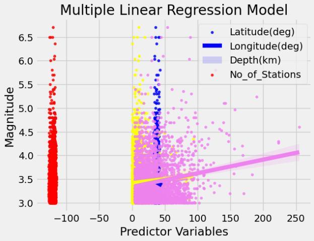
The linear regression model achieved an R² score of 0.035, indicating that it could explain only a small fraction of the variance in earthquake magnitudes. The relatively high MSE (0.175628) suggests that while the model provides a basic prediction, there is considerable room for improvement, particularly in accuracy.
Support vector machine
The SVM model performed poorly with an R² value of -1.92 and a high MSE of 0.531661. These results suggest that the model struggled to capture any meaningful relationship between the input features and the target variable, making it unsuitable for this task in its current form. Further hyperparameter tuning or feature engineering could improve its performance, but based on the current results, SVM is not ideal for this problem.
Random forest
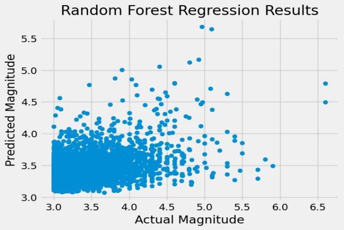
The Random Forest model emerged as the best performer, with the lowest MSE (0.155991) and the highest R² (0.142881) among the models tested. While the R² is still low, indicating that the model only explains a small part of the variance, its relatively lower MSE suggests that it is the most accurate model for predicting earthquake magnitudes. The ability of Random Forest to capture complex relationships in the data likely contributed to its superior performance compared to simpler models like Linear Regression and SVM.
Random forest classifier
This is an ensemble method that builds multiple decision trees on random data samples and features, combining their votes to improve accuracy and reduce overfitting. It is robust, handles large datasets, and reduces the risk of overfitting.
Table 3. Model scores.
This table is shown in the PDF version of the article.
Risk score and risk levels
Sample 1: Risk Score: 2.13.
Sample 1: Likelihoods={'Low': 0.0, 'Medium': 0.71, 'High': 0.29}, Consequences-Moderate damage, some injuries, potential economic losses, Risk Level=None, Risk Score: 2.13.
Sample 2: Risk Score: 2.8499999999999996.
Sample 2: Likelihoods={'Low': 0.0, 'Medium': 0.95, 'High': 0.05}, Consequences-Moderate damage, some injuries, potential economic losses, Risk Level=None, Risk Score: 2.849.
Sample 3: Risk Score: 2.94.
Sample 3: Likelihoods={'Low': 0.0, 'Medium': 0.98, 'High': 0.02}, Consequences-Moderate damage, some injuries, potential economic losses, Risk Level=None, Risk Score: 2.94.
Sample 4: Risk Score: 2.61.
Sample 4: Likelihoods={'Low': 0.0, 'Medium': 0.87, 'High': 0.13}, Consequences-Moderate damage, some injuries, potential economic losses, Risk Level=None, Risk Score: 2.61.
Sample 5: Risk Score: 2.55.
Sample 5: Likelihoods={'Low': 0.0, 'Medium': 0.85, 'High': 0.15}, Consequences-Moderate damage, some injuries, potential economic losses, Risk Level=None, Risk Score: 2.55.
5.2 Predicting Earthquake Prone Coordinates
5.2.1 Latitude and longitude earthquake-prone areas
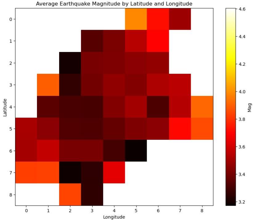
Divide the map into grids based on latitude and longitude. For each grid, calculate the average magnitude of earthquakes within it. Color the grids on a map: Hotter colors (reds, yellows) for grids with higher average magnitudes (more prone to strong earthquakes) and cooler colors (blues, greens) for grids with lower average magnitudes. This way, we can visually see which areas have experienced stronger earthquakes on average and might be considered more earthquake-prone.
6. Discussion
Linear Regression: while linear regression is a fundamental approach, its performance in this context highlights the challenges of using a simple model for a complex problem like earthquake magnitude prediction. The relatively high MSE indicates that the model fails to provide highly accurate forecasts. However, it still offers a basic understanding of the relationship between the features and the target variable.
6.1 Support Vector Machine
The negative R² score for the SVM model indicates that it performed worse than a simple mean-based prediction, suggesting that this method is unsuitable for the given task without further modifications. SVM might need additional feature transformation, parameter tuning, or even a different kernel to perform well in this domain. However, based on the current results, SVM's utility in this problem appears limited.
6.2 Random Forest
Despite the modest R² score, the Random Forest model outperformed the others by achieving the lowest MSE, making it the most accurate model for predicting earthquake magnitudes. This performance is likely due to the Random Forest's ability to handle non-linear relationships and capture complex interactions in the data. As an ensemble method, Random Forests combine multiple decision trees, which likely contribute to better prediction accuracy than linear models.
6.3 Gaussian Naive Bayes
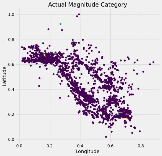
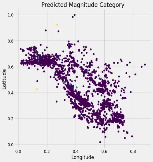
Useful for classifying magnitude types (e.g., minor, moderate, strong) with an accuracy rate of 70%, which could be improved with additional features.
6.4 The Random Forest Classifier
It is used for its ability to provide probabilistic predictions, handle complex relationships, and be robust to outliers. It helps quantify earthquake risk by predicting probabilities for different magnitude categories and identifying key features.
7. Conclusion
In this study, we applied ML models to predict earthquake magnitude using the earthquake dataset. Our findings reveal that the Random Forest model outperformed other methods, with the lowest MSE and highest R² value, underscoring its capability to capture intricate patterns in seismic data. This suggests ensemble models, particularly Random Forest, hold promise for earthquake magnitude prediction and Random Forest Classifiers for better risk assessment and prediction coordinates more prone to earthquakes. Future research might expand on this work by incorporating real-time seismic data and additional geological features. This could lead to more robust and responsive early warning systems, ultimately enhancing community preparedness and disaster mitigation efforts.
Data Availability
The data used in this study were sourced from the publicly accessible earthquake dataset. This dataset was utilized in its original form without any additional data generation. No new data were created during this study, and all relevant data can be accessed freely via the provided source.
Conflicts of Interest
The authors declare no conflict of interest. Funders played no role in the design of the study, data collection, analysis, or interpretation, nor in the writing of the manuscript or the decision to publish the results.
Appendix
Mathematical formulations and proofs
In this section, we provide the detailed mathematical formulations used in the paper's earthquake prediction models. These equations are fundamental to understanding how the different models were constructed and evaluated.
I. Richter scale formula: The magnitude M of an earthquake is defined using the Richter scale based on the amplitude A of seismic waves recorded by a seismograph and the distance (δ) from the seismic station to the earthquake's epicenter. The formula is given by: M = log10(A) − log10(A₀(δ)) where A₀(δ) is the standard amplitude for a zero-magnitude earthquake at a given distance.
II. Stress-strain relationship: Stress and strain are essential parameters in earthquake prediction models.
Hooke's Law gives the relationship between them: σ = E · ε where σ is the stress, E is the Young's modulus, and ε is the strain.
III. MSE: The MSE formula used to evaluate the model performance is: MSE = (1/n) Σ (yᵢ − ŷᵢ)² where yᵢ is the actual earthquake magnitude, and ŷᵢ is the predicted magnitude, with n being the total number of observations.
Additional figures and tables
This is an illustration of the network used to model seismic data. This network diagram highlights the relationships between key features such as location, depth, and magnitude.
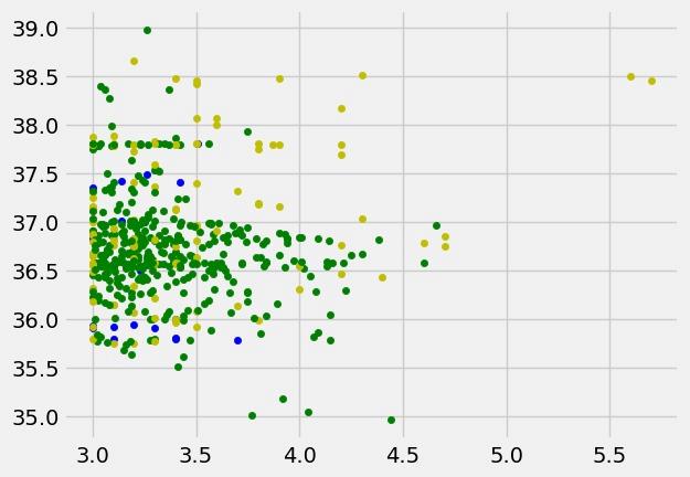
I. Visualization of earthquake events based on their magnitudes and locations, showing clusters of significant seismic activity in California between 2017 and 2019.
II. Overview of the dataset used in the study, including the number of records, the range of magnitudes, and key features like depth, latitude, and longitude.
Table A1. Description of key features used in the earthquake prediction models.
Feature Description Earthquake ID Unique identifier for each earthquake event Magnitude (M) Earthquake magnitude on the Richter scale Depth (D) Depth of the earthquake (in km) Latitude (Lat) Latitude of the earthquake epicenter Longitude (Lon) Longitude of the earthquake epicenter Seismic stations Number of stations reporting seismic activity
Experimental setup
This section provides additional technical details about the experimental setup for evaluating the performance of machine learning models.
Data preprocessing: The dataset used in this study was cleaned to remove any missing or irrelevant entries. The following preprocessing steps were applied:
I. Handling of missing values through imputation techniques.
II. Convert the date and time fields into a single datetime index to facilitate time-based analysis.
III. Feature scaling for certain variables, such as depth and magnitude, to ensure uniformity in model inputs. Model hyperparameters: For each machine learning model used in the experiment, the following hyperparameters were tuned:
I. Linear regression: No specific tuning is required, as it is a simple linear model.
II. Svm: The kernel function was chosen as the Radial Basis Function (RBF), with hyperparameters C and γ adjusted using grid search.
III. Naive bayes: The Gaussian Naive Bayes model was employed, with no specific tuning.
IV. Random forest regressor: The number of trees was set to 100, and the maximum depth of the trees was varied between 5 and 15.
Supplementary data
Dataset: The earthquake dataset, which includes earthquake records from 1966 to 2007, is available publicly. The dataset includes the key features used in this study, such as magnitude, depth, latitude, longitude, and time of occurrence.
Code: The Python code used to implement the machine learning models and data preprocessing steps is available for download.
References
- [1] Galkina, A., & Grafeeva, N. (2019). Machine learning methods for earthquake prediction: A survey. The Fourth conference on software engineering and information management (pp. 25-33). CEUR workshop proceedings. https://www.researchgate.net/publication/333774922
- [2] Mousavi, S. M., & Beroza, G. C. (2023). Machine learning in earthquake seismology. Annual review of earth and planetary sciences, 51(1), 105–129. https://doi.org/10.1146/annurev-earth-071822-100323
- [3] Sadhukhan, B., Chakraborty, S., & Mukherjee, S. (2023). Predicting the magnitude of an impending earthquake using deep learning techniques. Earth science informatics, 16(1), 803–823. https://doi.org/10.1007/s12145-022-00916-2
- [4] Iaccarino, A. G., Cristofaro, A., Picozzi, M., Spallarossa, D., & Scafidi, D. (2024). Real-time prediction of distance and PGA from P-wave features using gradient boosting regressor for on-site earthquake early warning applications. Geophysical journal international, 236(1), 675–687. https://doi.org/10.1093/gji/ggad443
- [5] Xu, Y., Yonghua, L., & Zengxi, G. (2021). Machine learning and its application in seismology. Reviews of geophysics and planetary physics, 52(1), 76–88. http://dx.doi.org/10.19975/j.dqyxx.2020-006
- [6] Anderson, R. N., Hasegawa, A., Umino, N., & Takagi, A. (1980). Phase changes and the frequency-magnitude distribution in the upper plane of the deep seismic zone beneath Tohoku, Japan. Journal of geophysical research: Solid earth, 85(B3), 1389–1398. https://doi.org/10.1029/JB085iB03p01389
- [7] Smith, D. E., Christodoulidis, D. C., Kolenkiewicz, R., Dunn, P. J., Klosko, S. M., Torrence, M. H., … ., & Blackwell, S. (1985). A global geodetic reference frame from LAGEOS ranging (SL5. 1AP). Journal of geophysical research: Solid earth, 90(B11), 9221–9233. https://doi.org/10.1029/JB090iB11p09221
- [8] Painter, O., Lee, R. K., Scherer, A., Yariv, A., O’brien, J. D., Dapkus, P. D., & Kim, I. (1999). Two-dimensional photonic band-gap defect mode laser. Science, 284(5421), 1819–1821. https://doi.org/10.1126/science.284.5421.1819
- [9] Paul, A., Gupta, S., Ghosh, S., & Choudhury, D. (2020). Probabilistic assessment and study of earthquake recurrence models for entire Northeast region of India. Natural hazards, 102, 15–45. https://doi.org/10.1007/s11069-020-03909-w
- [10] Zhu, W., & Beroza, G. C. (2019). PhaseNet: A deep-neural-network-based seismic arrival-time picking method. Geophysical journal international, 216(1), 261–273. https://doi.org/10.1093/gji/ggy423
- [11] Chen, Y., Zhang, M., Bai, M., & Chen, W. (2019). Improving the signal-to-noise ratio of seismological datasets by unsupervised machine learning. Seismological research letters, 90(4), 1552–1564. https://doi.org/10.1785/0220190028
- [12] Zhang, J., Yi, S., Liang, G. U. O., Hongli, G. A. O., Xin, H., & Hongliang, S. (2020). A new bearing fault diagnosis method based on modified convolutional neural networks. Chinese journal of aeronautics, 33(2), 439–447. https://doi.org/10.1016/j.cja.2019.07.011
- [13] Patel, D., Arcomano, T., Hunt, B., Szunyogh, I., & Ott, E. (2024). Exploring the potential of hybrid machine-learning/physics-based modeling for atmospheric/oceanic prediction beyond the medium range. https://doi.org/10.48550/arXiv.2405.19518
- [14] Hao, X., Liu, L., Yang, R., Yin, L., Zhang, L., & Li, X. (2023). A review of data augmentation methods of remote sensing image target recognition. Remote sensing, 15(3), 827. https://doi.org/10.3390/rs15030827
- [15] Ju, Y. J., Park, J. H., & Lee, S. W. (2023). NeuroInspect: Interpretable neuron-based debugging framework through class-conditional visualizations. https://doi.org/10.48550/arXiv.2310.07184
- [16] Hong, S. J., Kim, H. M., Huh, D., Suryanarayana, C., & Chun, B. S. (2003). Effect of clustering on the mechanical properties of SiC particulate-reinforced aluminum alloy 2024 metal matrix composites. Materials science and engineering: A, 347(1–2), 198–204. https://doi.org/10.1016/S0921-5093(02)00593-2
- [17] Kumar, S., & Singh, B. (2024). Intelligent learning model in adaptive e-learning and evaluation framework. Machine intelligence research, 18(1), 226–238. https://machineintelligenceresearchs.com/index.php/mir/article/view/19
- [18] Zhang, Q., Liu, X., Zhang, H., Xu, C., Yang, G., Yuan, Y., Gao, Z. (2024). Variational field constraint learning for degree of coronary artery ischemia assessment. International conference on medical image computing and computer-assisted intervention (pp. 768–778). Springer. https://doi.org/10.1007/978-3-031-72384-1_72
- [19] Yoon, C. E., O’Reilly, O., Bergen, K. J., & Beroza, G. C. (2015). Earthquake detection through computationally efficient similarity search. Science advances, 1(11), e1501057. https://doi.org/10.1126/sciadv.1501057
- [20] Kong, Q., Trugman, D. T., Ross, Z. E., Bianco, M. J., Meade, B. J., & Gerstoft, P. (2019). Machine learning in seismology: Turning data into insights. Seismological research letters, 90(1), 3–14. https://doi.org/10.1785/0220180259
- [21] Xie, Y., Ebad Sichani, M., Padgett, J. E., & DesRoches, R. (2020). The promise of implementing machine learning in earthquake engineering: A state-of-the-art review. Earthquake spectra, 36(4), 1769–1801. https://doi.org/10.1177/8755293020919419
- [22] Buscema, M., & Ruggieri, M. (2011). Advanced networks, algorithms and modeling for earthquake prediction (Vol. 12). River Publishers. https://B2n.ir/ux4771
- [23] Mignan, A., & Chen, C. C. (2016). The spatial scale of detected seismicity. Pure and applied geophysics, 173, 117–124. https://doi.org/10.1007/s00024-015-1133-7
- [24] Dikmen, O. (2024). Comparative analysis of machine learning models for earthquake prediction: A case study of Düzce, Türkiye. International journal of innovative research in engineering and management, 11(5), 73-
- [82] https://doi.org/10.55524/ijirem.2024.11.5.10